Salt la conținutul principal

Cum să căutați și să returnați mai multe valori corespunzătoare pe orizontală în Excel?

doc-vlookup-orizontal-1
În mod implicit, funcția VLOOKUP poate returna mai multe valori corespunzătoare la nivel vertical în Excel, în unele cazuri, poate doriți să returnați mai multe valori la nivel orizontal, așa cum este prezentat mai jos. Aici vă voi spune că o formulă poate rezolva această sarcină.
VLOOKUP și returnează mai multe valori pe orizontală

săgeată albastru dreapta balon VLOOKUP și returnează mai multe valori pe orizontală

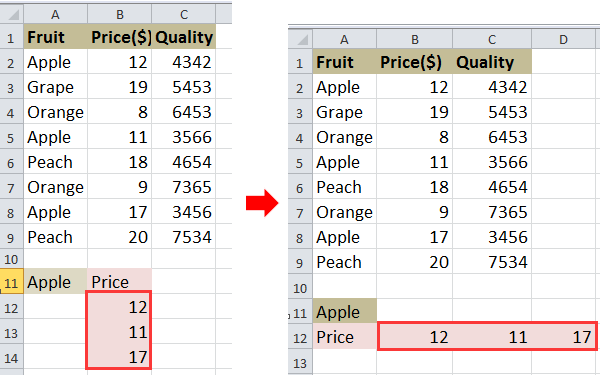
De exemplu, aveți o gamă de date, așa cum este prezentată mai jos, și doriți să căutați prețurile Apple.
doc-vlookup-orizontal-2

1. Selectați o celulă și tastați această formulă =INDEX($B$2:$B$9, SMALL(IF($A$11=$A$2:$A$9, ROW($A$2:$A$9)-ROW($A$2)+1), COLUMN(A1))) și apoi apăsați Shift + Ctrl + Enter și trageți mânerul de completare automată spre dreapta pentru a aplica această formulă până la #PE UNU! apare. Vedeți captura de ecran:
doc-vlookup-orizontal-3

2. Apoi ștergeți #NUM !. Vedeți captura de ecran:
doc-vlookup-orizontal-4

Sfat: În formula de mai sus, B2: B9 este intervalul de coloane în care doriți să returnați valorile, A2: A9 este intervalul de coloane în care se află valoarea de căutare, A11 este valoarea de căutare, A1 este prima celulă din intervalul dvs. de date , A2 este prima celulă din intervalul de coloane în care se află valoarea de căutare.

Dacă doriți să returnați mai multe valori pe verticală, puteți citi acest articol Cum să căutați valoarea returnează mai multe valori corespunzătoare în Excel?


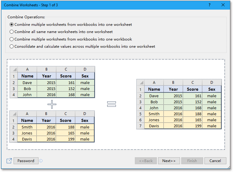
Combinați cu ușurință mai multe foi / registru de lucru într-o singură coală sau registru de lucru

Pentru a combina mai multe foi sau registre de lucru într-o singură foaie sau registru de lucru poate fi dificil în Excel, dar cu Combina funcție în Kutools pentru Excel, puteți combina fuzionarea a zeci de foi / registre de lucru într-o singură foaie sau registru de lucru, de asemenea, puteți consolida foile într-una numai cu câteva clicuri.  Faceți clic pentru o versiune de încercare gratuită de 30 de zile!
combina foi
 
Kutools pentru Excel: cu peste 300 de programe de completare la îndemână Excel, gratuit pentru a încerca fără limitări în 30 de zile.

Cele mai bune instrumente de productivitate de birou

🤖 Kutools AI Aide: Revoluționați analiza datelor pe baza: Execuție inteligentă   |  Generați codul  |  Creați formule personalizate  |  Analizați datele și generați diagrame  |  Invocați funcțiile Kutools...
Caracteristici populare: Găsiți, evidențiați sau identificați duplicatele   |  Ștergeți rândurile goale   |  Combinați coloane sau celule fără a pierde date   |   Rundă fără Formula ...
Super căutare: VLookup cu mai multe criterii    VLookup cu valori multiple  |   VLookup pe mai multe foi   |   Căutare fuzzy ....
Listă derulantă avansată: Creați rapid o listă derulantă   |  Listă drop-down dependentă   |  Listă derulantă cu selectare multiplă ....
Manager de coloane: Adăugați un număr specific de coloane  |  Mutați coloanele  |  Comutați starea vizibilității coloanelor ascunse  |  Comparați intervale și coloane ...
Caracteristici prezentate: Focus pe grilă   |  Vedere de proiectare   |   Big Formula Bar    Manager registru de lucru și foi   |  Biblioteca de resurse (Text automat)   |  Data Picker   |  Combinați foi de lucru   |  Criptare/Decriptare celule    Trimiteți e-mailuri după listă   |  Super Filtru   |   Filtru special (filtrează bold/italic/barat...) ...
Top 15 seturi de instrumente12 Text Instrumente (Adăuga text, Eliminați caractere,...)   |   50+ Diagramă Tipuri de (Gantt Chart,...)   |   40+ Practic Formule (Calculați vârsta pe baza zilei de naștere,...)   |   19 inserare Instrumente (Introduceți codul QR, Inserați imaginea din cale,...)   |   12 Convertire Instrumente (Numere la cuvinte, conversie valutara,...)   |   7 Merge & Split Instrumente (Rânduri combinate avansate, Celule divizate,...)   |   ... și altele

Îmbunătățiți-vă abilitățile Excel cu Kutools pentru Excel și experimentați eficiența ca niciodată. Kutools pentru Excel oferă peste 300 de funcții avansate pentru a crește productivitatea și a economisi timp.  Faceți clic aici pentru a obține funcția de care aveți cea mai mare nevoie...

Descriere


Fila Office aduce interfața cu file în Office și vă face munca mult mai ușoară

  • Activați editarea și citirea cu file în Word, Excel, PowerPoint, Publisher, Access, Visio și Project.
  • Deschideți și creați mai multe documente în filele noi ale aceleiași ferestre, mai degrabă decât în ​​ferestrele noi.
  • Vă crește productivitatea cu 50% și reduce sute de clicuri de mouse pentru dvs. în fiecare zi!
Comments (20)
No ratings yet. Be the first to rate!
This comment was minimized by the moderator on the site
This article says this uses VLOOKUP, but it uses INDEX... which does not help me. I need a solution for multiple values using VLOOKUP or XLOOKUP in tables.
This comment was minimized by the moderator on the site
you can use TEXTSPLIT function followed by TEXTJOIN FUNCTION in excel 365
This comment was minimized by the moderator on the site
For anyone experiencing issues in a big data range, ensure you dont have any cells existent with "#N/A" or it will break it. Simple error but can be overlooked.
This comment was minimized by the moderator on the site
Hello, I want to use keyword instead of specific text or value here for multiple return values, can you please share code formula for same.
This comment was minimized by the moderator on the site
Hello - This formula worked perfectly - thank you! However, I want to apply it to a long list of lookup values. When I copy and paste the formula it obviously returns the same results as the first lookup value so I removed the $'s from $A$11, but that changes the result to something incorrect. How can I quickly apply this same formula for a long list of lookup values?

Thank you!

M
This comment was minimized by the moderator on the site
Bonjour,

J'ai retransposé mon problème exactement dans les mêmes positions de colonne que l'exemple et j’obtiens le message #VALEUR! dès la première case.

Mon excel fonctionne en francais, j'ai tout retranscrit en francais, passé ";"au lieu de ",", appuyé sur CTRL+MAJ+Entrée... des idées sur l'origine du problème?

Fanny
This comment was minimized by the moderator on the site
what you want to put the price in order of highest qty from column c?
This comment was minimized by the moderator on the site
i have to find vertical value first, in vertical value there are more horizontal value and i have choose grater value which i have. which function or formula can help
This comment was minimized by the moderator on the site
Hi. I have three google spreadsheet. First sheet is named "Summary. It is a table containing the name of our employee and number of evaluation in a week from 1-7. The next sheet is named "Chat Score"and third sheet is named Ëmail Score". What I want to to do is when we input a evaluation score to one of our employee it will be automatically recorded on the "Summary sheet" as evaluation 1 or 2 and so on and so forth. In short I want to get multiple return value in a single seach key across multiple sheet. I hope you can help. https://docs.google.com/spreadsheets/d/1lt-e4MxddUKg5xDt_0YchBiEgGe4mFKB-dHENwwtA6Y/edit?usp=sharing

https://docs.google.com/spreadsheets/d/1lt-e4MxddUKg5xDt_0YchBiEgGe4mFKB-dHENwwtA6Y/edit?usp=sharing
This comment was minimized by the moderator on the site
Although I'm looking up my values in another worksheet (I don't think this should cause a problem?), I only seem to have success dragging to the right if I go in and change the +1 to '0' for the 1st instance of the lookup ID, '1' for the 2nd instance and so on. I know how many instances of the lookup ID I have so I can workaround. What do I need to change to allow me to successfully drag the fx across horizontally without needing to edit (i.e getting the #NUM to appear once there are no more lookup values to return).
This comment was minimized by the moderator on the site
Sorry, I have not found any solutions about your problems. If you have found that, could you tell me? Thank u.
This comment was minimized by the moderator on the site
Change Column to Row at the end of the formula

"=INDEX($B$1:$B$206, SMALL(IF($A$209=$A$1:$A$206, ROW($A$1:$A$206)-ROW($A$1)+1), ROW(A1)))"
This comment was minimized by the moderator on the site
How to List all values(like list of groceries bought) caused by a specific value (by a person X) using VLOOK_UP and other possible formulas
This comment was minimized by the moderator on the site
You mean that to list all grocerise a person need to buy, right? If so, you can refer to the formula in this article, and change the arguments as you need as below screenshot shown.
There are no comments posted here yet
Load More
Please leave your comments in English
Posting as Guest
×
Rate this post:
0   Characters
Suggested Locations