Salt la conținutul principal

Cum să sumați pe baza criteriilor de coloană și rând în Excel? 

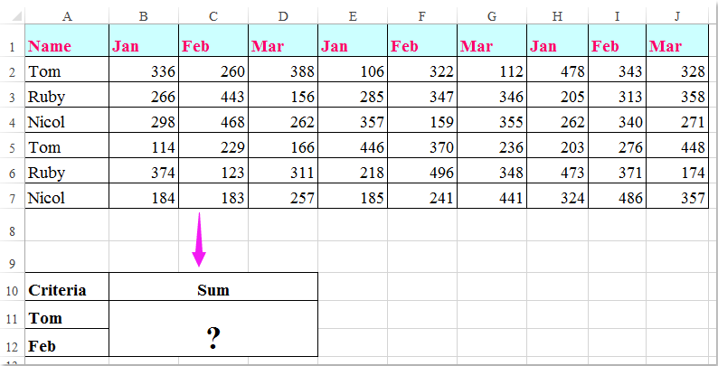
Am o serie de date care conțin anteturi de rânduri și coloane, acum vreau să iau o sumă de celule care îndeplinesc atât criteriile antetului coloanei, cât și ale rândurilor. De exemplu, pentru a rezuma celulele care criteriu de coloană este Tom și criteriile de rând sunt Feb, după cum se arată în următoarea captură de ecran. În acest articol, voi vorbi despre câteva formule utile pentru a-l rezolva.

criterii rând rând coloană sumă doc

Suma celulelor pe baza criteriilor de coloană și rând cu formule


săgeată albastru dreapta balon Suma celulelor pe baza criteriilor de coloană și rând cu formule

Aici puteți aplica următoarele formule pentru a însuma celulele pe baza atât a criteriilor coloanei, cât și a rândurilor, vă rugăm să faceți acest lucru:

Introduceți oricare dintre formulele de mai jos într-o celulă goală în care doriți să scoateți rezultatul:

=SUMPRODUCT((A2:A7="Tom")*(B1:J1="Feb")*(B2:J7))

=SUM(IF(B1:J1="Feb",IF(A2:A7="Tom",B2:J7)))

Și apoi apăsați Shift + Ctrl + Enter tastele împreună pentru a obține rezultatul, vezi captura de ecran:

criterii rând rând coloană sumă doc

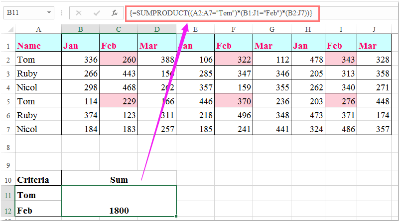
notițe: În formulele de mai sus: Tom și februarie sunt criteriile de coloană și rând pe care se bazează, A2: A7, B1: J1 sunt anteturile de coloană și anteturile de rând conțin criteriile, B2: J7 este intervalul de date pe care doriți să îl însumați.

Cele mai bune instrumente de productivitate de birou

🤖 Kutools AI Aide: Revoluționați analiza datelor pe baza: Execuție inteligentă   |  Generați codul  |  Creați formule personalizate  |  Analizați datele și generați diagrame  |  Invocați funcțiile Kutools...
Caracteristici populare: Găsiți, evidențiați sau identificați duplicatele   |  Ștergeți rândurile goale   |  Combinați coloane sau celule fără a pierde date   |   Rundă fără Formula ...
Super căutare: VLookup cu mai multe criterii    VLookup cu valori multiple  |   VLookup pe mai multe foi   |   Căutare fuzzy ....
Listă derulantă avansată: Creați rapid o listă derulantă   |  Listă drop-down dependentă   |  Listă derulantă cu selectare multiplă ....
Manager de coloane: Adăugați un număr specific de coloane  |  Mutați coloanele  |  Comutați starea vizibilității coloanelor ascunse  |  Comparați intervale și coloane ...
Caracteristici prezentate: Focus pe grilă   |  Vedere de proiectare   |   Big Formula Bar    Manager registru de lucru și foi   |  Biblioteca de resurse (Text automat)   |  Data Picker   |  Combinați foi de lucru   |  Criptare/Decriptare celule    Trimiteți e-mailuri după listă   |  Super Filtru   |   Filtru special (filtrează bold/italic/barat...) ...
Top 15 seturi de instrumente12 Text Instrumente (Adăuga text, Eliminați caractere,...)   |   50+ Diagramă Tipuri de (Gantt Chart,...)   |   40+ Practic Formule (Calculați vârsta pe baza zilei de naștere,...)   |   19 inserare Instrumente (Introduceți codul QR, Inserați imaginea din cale,...)   |   12 Convertire Instrumente (Numere la cuvinte, conversie valutara,...)   |   7 Merge & Split Instrumente (Rânduri combinate avansate, Celule divizate,...)   |   ... și altele

Îmbunătățiți-vă abilitățile Excel cu Kutools pentru Excel și experimentați eficiența ca niciodată. Kutools pentru Excel oferă peste 300 de funcții avansate pentru a crește productivitatea și a economisi timp.  Faceți clic aici pentru a obține funcția de care aveți cea mai mare nevoie...

Descriere


Fila Office aduce interfața cu file în Office și vă face munca mult mai ușoară

  • Activați editarea și citirea cu file în Word, Excel, PowerPoint, Publisher, Access, Visio și Project.
  • Deschideți și creați mai multe documente în filele noi ale aceleiași ferestre, mai degrabă decât în ​​ferestrele noi.
  • Vă crește productivitatea cu 50% și reduce sute de clicuri de mouse pentru dvs. în fiecare zi!
Comments (17)
No ratings yet. Be the first to rate!
This comment was minimized by the moderator on the site
Brilliant!

The function =SUM(IF(B1:J1="Feb",IF(A2:A7="Tom",B2:J7))) is a great X & Y summation tool.
I would not have thought this logic out on my own.
In fact i took me a minute to deconstruction the operations.

Thank you
This comment was minimized by the moderator on the site
My data that I am trying to retrieve is in a table. Would this impact the result at all? I have:

=SUM(IF('[Primary Controller Active Project Database (KC notes)1.xlsx]Active Project Tracking'!$B2:$B66=X2,IF('[Primary Controller Active Project Database (KC notes)1.xlsx]Active Project Tracking'!$A1:$AV1=AH10,'[Primary Controller Active Project Database (KC notes)1.xlsx]Active Project Tracking'!$H$2:$AV$66)))

So I think the equivalent would be if you did your information above, but in a table in a different workbook. Thoughts?
This comment was minimized by the moderator on the site
If there were negatives in the matrix and you only wanted to include the positives, what would you do? 
I tried to do something like this:

=SUMPRODUCT((Column = Criteria)* ( Row = Criteria) * (second column = Criteria) * (Matrix) * (Matrix >0))

This comment was minimized by the moderator on the site
Is there a way to do this but instead of writing "Tom" & "Feb" in the formula, you are able to reference the criteria cells e.g.A11 & A12?
This comment was minimized by the moderator on the site
Hello, Rianna,Yest, as you said, you can use the cell references to replace the text in the formula, such as:
=SUMPRODUCT((A2:A7=A2)*(B1:J1=C1)*(B2:J7))
=SUM(IF(B1:J1=C1,IF(A2:A7=A2,B2:J7)))
This comment was minimized by the moderator on the site
In the above example which formula should I use if I wanted calculate the sum of the amounts earned by Tom Ruby & Nicol in March?
This comment was minimized by the moderator on the site
Hello, Nabar,To get the result you want, please apply the below formula:=SUMPRODUCT(((A2:A7="Tom")+(A2:A7="Nicol")+(A2:A7="Ruby"))*(B1:J1="Mar")*(B2:J7))
Please try, hope it can help you!
This comment was minimized by the moderator on the site
Hello Skyyang,
Thank you for your response. I tried the formula you suggested but I am not getting the right answer. Probably I wasn't able to put my query correctly. Let me try again I have a spreadsheet with data with daily calculation, I have numbered the first row 1,2,3,4.....132. 2nd, 3rd 4th &5th rows has table headings. The first column has line no's numbered 1, 2,3,.....3005 starting from row 6,range B6:EF3005 has data filled in on everyday basis. In second sheet i have a table in which I want to apply a formula which will look up two line numbers fed in two different rows and calculate the sum from the range B6: EF3005 from the data spreadsheet between the two line numbers from a certain column viz sum of values in column 15 between rows (line No's) 50 & 85.
This comment was minimized by the moderator on the site
Is there a way to make this work with wildcard characters? I'd like to use it on everything starting with certain characters, but with (a fixed number of) undefined characters at the end, i.e. =SUM(IF(B1:J1="Fe*",IF(A2:A7="To*",B2:J7)))
This comment was minimized by the moderator on the site
Should anyone have the same question, this is how I solved it (in Google Sheets, not tested in Excel):

=ArrayFormula(SUM(IF(regexmatch(O5:W5,"^Fe."),IF(regexmatch(N6:N11,"^To."),O6:W11))))

Note that the IF function does not support wildcard characters and that for regexmatch the wildcards are different and can be found here: https://github.com/google/re2/blob/master/doc/syntax.txt
In this particular instance, I used ^ to indicate that Fe & Tom occur at the beginning of text and . to allow for any following character (* would mean zero or more of the previous character, e.g. Fe* would only look for instances with 1 or more "e"s after F)
This comment was minimized by the moderator on the site
I tried to create a formula to calculate if the D12 is blank, it will calculate from K12 to AH12 but it seems this part ' regexmatch(D12,"")' is not working
ArrayFormula(SUM(IF(regexmatch(D12,""),K12:AH12)))
This comment was minimized by the moderator on the site
Thank you so much! You made my day!! @TeSageDS
This comment was minimized by the moderator on the site
how would you do this same formula if you wanted to sum both Feb and March together? please help! thanks

=SUMPRODUCT((A2:A7="Tom")*(B1:J1="Feb")*(B2:J7))
This comment was minimized by the moderator on the site
Hello,Angela,
To solve your problem, you just need to apply the below formula, please try it.

=SUMPRODUCT((A2:A7="Tom")*((B1:J1="Feb")+(B1:J1="Mar"))*(B2:J7)).

Hope it can help you!
This comment was minimized by the moderator on the site
Brilliant
This comment was minimized by the moderator on the site
Worth pointing out that of the two formulas provided above you do not need to enter the SUMPRODUCT formula with Ctrl + Shift + Enter. It will work perfectly well without it.
This comment was minimized by the moderator on the site
Awesome, this is the one what i was looking for. thanks for the help
There are no comments posted here yet
Please leave your comments in English
Posting as Guest
×
Rate this post:
0   Characters
Suggested Locations