Salt la conținutul principal

Cum se creează o listă verticală dependentă în foaia Google?

Introducerea listei derulante normale în foaia Google poate fi o treabă ușoară pentru dvs., dar, uneori, poate fi necesar să introduceți o listă derulantă dependentă, ceea ce înseamnă a doua listă derulantă în funcție de alegerea primei listă derulantă. Cum ați putea face față acestei sarcini în foaia Google?

Creați o listă verticală dependentă în foaia Google


Creați o listă verticală dependentă în foaia Google

Următorii pași vă pot ajuta să inserați o listă verticală dependentă, vă rugăm să procedați astfel:

1. Mai întâi, ar trebui să inserați lista verticală de bază, selectați o celulă în care doriți să puneți prima listă verticală, apoi faceți clic pe Date > Data validarii, vezi captura de ecran:

2. În pop-out Data validarii fereastră de dialog, selectați Lista dintr-o gamă din lista derulantă de lângă Criterii , apoi faceți clic pe buton pentru a selecta valorile celulei pe care doriți să creați prima listă derulantă pe baza, vedeți captura de ecran:

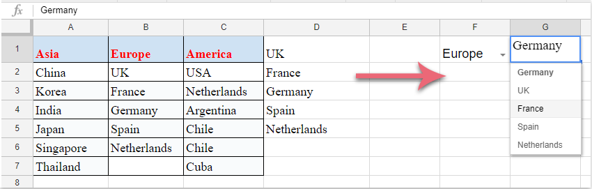
3. Apoi apasa Economisiți butonul, a fost creată prima listă derulantă. Alegeți un articol din lista verticală creată, apoi introduceți această formulă: =arrayformula(if(F1=A1,A2:A7,if(F1=B1,B2:B6,if(F1=C1,C2:C7,"")))) într-o celulă necompletată adiacentă coloanelor de date, apoi apăsați Intrați tasta, toate valorile potrivite bazate pe primul element din lista derulantă au fost afișate simultan, consultați captura de ecran:

notițe: În formula de mai sus: F1 este prima celulă din lista derulantă, A1, B1 și C1 sunt elementele din prima listă derulantă, A2: A7, B2: B6 și C2: C7 sunt valorile celulei pe care se bazează a doua listă derulantă. Îi poți schimba pe ai tăi.

4. Și apoi puteți crea a doua listă verticală dependentă, faceți clic pe o celulă în care doriți să puneți a doua listă verticală, apoi faceți clic pe Date > Data validarii a merge la Data validarii caseta de dialog, alegeți Lista dintr-o gamă din meniul derulant de lângă Criterii secțiunea și continuați să faceți clic pe buton pentru a selecta celulele de formulă care sunt rezultatele potrivite ale primului element derulant, consultați captura de ecran:

5. În cele din urmă, faceți clic pe butonul Salvare, iar a doua listă verticală dependentă a fost creată cu succes, după cum se arată în următoarea captură de ecran:

Cele mai bune instrumente de productivitate de birou

🤖 Kutools AI Aide: Revoluționați analiza datelor pe baza: Execuție inteligentă   |  Generați codul  |  Creați formule personalizate  |  Analizați datele și generați diagrame  |  Invocați funcțiile Kutools...
Caracteristici populare: Găsiți, evidențiați sau identificați duplicatele   |  Ștergeți rândurile goale   |  Combinați coloane sau celule fără a pierde date   |   Rundă fără Formula ...
Super căutare: VLookup cu mai multe criterii    VLookup cu valori multiple  |   VLookup pe mai multe foi   |   Căutare fuzzy ....
Listă derulantă avansată: Creați rapid o listă derulantă   |  Listă drop-down dependentă   |  Listă derulantă cu selectare multiplă ....
Manager de coloane: Adăugați un număr specific de coloane  |  Mutați coloanele  |  Comutați starea vizibilității coloanelor ascunse  |  Comparați intervale și coloane ...
Caracteristici prezentate: Focus pe grilă   |  Vedere de proiectare   |   Big Formula Bar    Manager registru de lucru și foi   |  Biblioteca de resurse (Text automat)   |  Data Picker   |  Combinați foi de lucru   |  Criptare/Decriptare celule    Trimiteți e-mailuri după listă   |  Super Filtru   |   Filtru special (filtrează bold/italic/barat...) ...
Top 15 seturi de instrumente12 Text Instrumente (Adăuga text, Eliminați caractere,...)   |   50+ Diagramă Tipuri de (Gantt Chart,...)   |   40+ Practic Formule (Calculați vârsta pe baza zilei de naștere,...)   |   19 inserare Instrumente (Introduceți codul QR, Inserați imaginea din cale,...)   |   12 Convertire Instrumente (Numere la cuvinte, conversie valutara,...)   |   7 Merge & Split Instrumente (Rânduri combinate avansate, Celule divizate,...)   |   ... și altele

Îmbunătățiți-vă abilitățile Excel cu Kutools pentru Excel și experimentați eficiența ca niciodată. Kutools pentru Excel oferă peste 300 de funcții avansate pentru a crește productivitatea și a economisi timp.  Faceți clic aici pentru a obține funcția de care aveți cea mai mare nevoie...

Descriere


Fila Office aduce interfața cu file în Office și vă face munca mult mai ușoară

  • Activați editarea și citirea cu file în Word, Excel, PowerPoint, Publisher, Access, Visio și Project.
  • Deschideți și creați mai multe documente în filele noi ale aceleiași ferestre, mai degrabă decât în ​​ferestrele noi.
  • Vă crește productivitatea cu 50% și reduce sute de clicuri de mouse pentru dvs. în fiecare zi!
Comments (18)
No ratings yet. Be the first to rate!
This comment was minimized by the moderator on the site
Hi there. Its been working but for it only appears that only one cell can be formulated.I need help 
For example: in Cell A1, it shows dependent dropdown, but when in cell a2 it does not work.
Thas what help that i need, From A:A, They have all different selection from the dropdown list. Thanks.
This comment was minimized by the moderator on the site
Would it been possible to create pull down menu based of formula?
I use formula "=SUMIFS(Items!$I:$I,Items!$A:$A,K$1,Items!$D:$D,$D2)" (=for example 150) to find the qty on pallet based on item and container size.
So I wanted to create pull down menu like qty 1 pallet, qty 2 pallets, qty 3 pallets,.....
Then user will always order qty of full pallets like 150, 2 x 150, 3 x150, up to 21 x 150.
This comment was minimized by the moderator on the site
Hi, I already created a drop down list like this one, what I'd like to know is how i can, when clicking on one option from that list, restrict what appears as options on another cell. For example, in one cell i can choose between laparoscopy and orthopaedics. If I choose orthopaedics then, the other cell which has a list of doctors, should only show the doctors for orthopedy and not all of them. Does anyone know how to do this?
This comment was minimized by the moderator on the site
Hii Sir,
I Want to Create A Dependent Drop Down List Like
- State(A1):- District(B1):- Taluka(C1) :- Then Information(D1) ,
So I need your Help .
Tell How do you do this Type of Dependent Drop down List in Excel or Google Sheet
This comment was minimized by the moderator on the site
Hi, Shelate,
Maybe the below article can solve your problem, please view it:
https://www.extendoffice.com/documents/excel/5852-excel-multiple-level-drop-down-list.html

Please try, hope it can help you!
This comment was minimized by the moderator on the site
Now is needed to use: =arrayformula(if(F1=A1;A2:A7;if(F1=B1;B2:B6;if(F1=C1;C2:C7;""))))
This comment was minimized by the moderator on the site
Thank you soooo much!
This comment was minimized by the moderator on the site
Hi,
I was wondering if anyone could advise me with this? I've followed the above steps but on step 3 rather than getting:
"...all the matching values based on the first drop down list item have been displayed at once," I am just seeing one value (the top one from the drop down list).
My cells are placed slightly differently and the first drop down is filled from another sheet (from anywhere int eh column excluding the top row) so my formula is:

=arrayformula(if(VLE!D2:D=B11,B12,if(VLE!D2:D=C11,C12:C14,if(VLE!D2:D=D11,D12:D14,if(VLE!D2:D=E11,E12:E16,if(VLE!D2:D=F11,F12:F16,""))))))

It is correctly displaying the top drop down option for each of (using cell numbers from the step 3 example on this page) A1, B1, and C1 so, again using this page's example, if I select Asia form the F1 drop down, I would get China, but nothing further


Any suggestions?

Many thanks! Nick
This comment was minimized by the moderator on the site
If the first drop own is on sheet 1 A1, will this work were I want the second drop down as sheet 1 A2, but to have its data range on a separate sheet?
This comment was minimized by the moderator on the site
Ich bekomm immer die Meldung "Fehler beim Parsen der Formel" wenn ich =arrayformula(if(F1=A1,A2:A7,if(F1=B1,B2:B6,if(F1=C1,C2:C7,"")))) eingebe. Was ist der "Weiter-Schlüsel"? Reicht es nicht wie bei Excel die Formel einzugeben?
This comment was minimized by the moderator on the site
Ersetzen Sie den , zu ;
es hat für mich funktioniert
This comment was minimized by the moderator on the site
This is the best explanation I have found, so thank you for that!

In my situation, I am working with over 200 rows with more being continuously added. Is there an easier/more efficient way to handle this many rows?
This comment was minimized by the moderator on the site
Yes, if you don't put number index to specify ending cell.
Like instead of C2:C7 you put C2:C. This will automatically tell the array formula, that you want to consider all values in column "C" starting at "C2".
This comment was minimized by the moderator on the site
What happens if I want exactly the same dropdown list in F2 as you have in F1 ?
I tried, and it doesn't overwrite D1:D7 .. meaning D1:D7 is only available once.
I need something else, double dropdown, but on many-many lines .. guess I must use another system then .. not sure which ..
This comment was minimized by the moderator on the site
Hi, Xained,
This method can only applied to one cell, if you have some good ways for applying this to multiple cells, please comment here.

Thank you!
This comment was minimized by the moderator on the site
Please, guide me how to do that.Thanks
This comment was minimized by the moderator on the site
혹시, 하나의 셀이 아닌 여러셀에 할 수 있는 방법을 알 수 있을까요?
This comment was minimized by the moderator on the site
내말이... 시바 좃빠지게 따라했디만 밑에줄은 안되노..
There are no comments posted here yet
Please leave your comments in English
Posting as Guest
×
Rate this post:
0   Characters
Suggested Locations