Cum se formată condiționat pe o altă foaie din foaia Google?
Dacă doriți să aplicați formatarea condiționată pentru a evidenția celulele pe baza unei liste de date dintr-o altă foaie, după cum urmează captura de ecran prezentată în foaia Google, aveți vreo metodă ușoară și bună pentru rezolvarea acesteia?
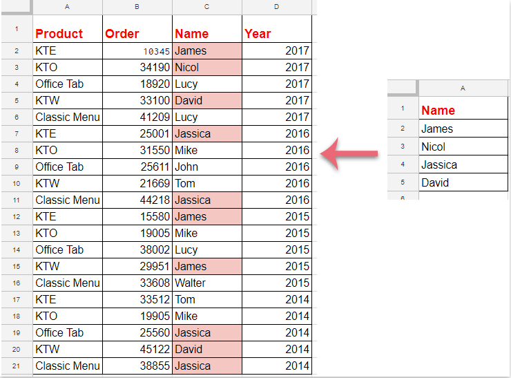
Formatare condiționată pentru a evidenția celulele pe baza unei liste dintr-o altă foaie din Foi de calcul Google

Vă rugăm să parcurgeți pașii următori pentru a finaliza această lucrare:
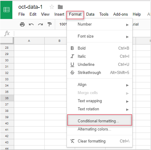
1. Clic Format > Formatarea condițională, vezi captura de ecran:
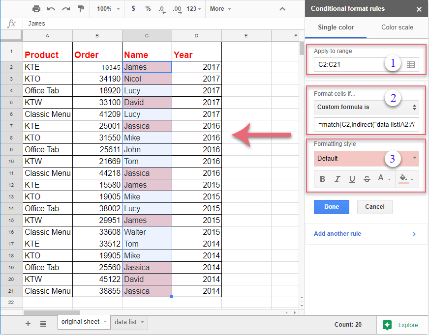
2. În Reguli de condiționare a formatului , faceți următoarele operații:
(1.) Faceți clic pe  buton pentru a selecta datele coloanei pe care doriți să le evidențiați;
(2.) În Formatați celulele dacă lista derulantă, vă rugăm să alegeți Formula personalizată este , apoi introduceți această formulă: = potrivire (C2, indirectă („listă de date! A2: A”), 0) în caseta de text;
(3.) Apoi selectați o formatare din Stil de formatare după cum ai nevoie.
notițe: În formula de mai sus: C2 este prima celulă a datelor coloanei pe care doriți să o evidențiați și lista de date! A2: A este numele foii și lista de celule de listă care conține criteriile pe care doriți să le evidențiați pe baza celulelor.
3. Și toate celulele potrivite bazate pe celulele listei au fost evidențiate simultan, apoi ar trebui să faceți clic pe Terminat pentru a închide butonul Reguli de condiționare a formatului panoul după cum aveți nevoie.
Cele mai bune instrumente de productivitate de birou
Îmbunătățiți-vă abilitățile Excel cu Kutools pentru Excel și experimentați eficiența ca niciodată. Kutools pentru Excel oferă peste 300 de funcții avansate pentru a crește productivitatea și a economisi timp. Faceți clic aici pentru a obține funcția de care aveți cea mai mare nevoie...
")
Fila Office aduce interfața cu file în Office și vă face munca mult mai ușoară
- Activați editarea și citirea cu file în Word, Excel, PowerPoint, Publisher, Access, Visio și Project.
- Deschideți și creați mai multe documente în filele noi ale aceleiași ferestre, mai degrabă decât în ferestrele noi.
- Vă crește productivitatea cu 50% și reduce sute de clicuri de mouse pentru dvs. în fiecare zi!
")