Salt la conținutul principal

Cum se returnează mai multe valori de potrivire bazate pe unul sau mai multe criterii în Excel?

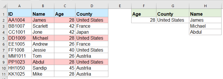
În mod normal, căutarea unei valori specifice și returnarea articolului care se potrivește este ușor pentru majoritatea dintre noi utilizând funcția VLOOKUP. Dar, ați încercat vreodată să returnați mai multe valori potrivite pe baza unuia sau mai multor criterii, după cum se arată în următoarea captură de ecran? În acest articol, voi introduce câteva formule pentru rezolvarea acestei sarcini complexe în Excel.

Returnează mai multe valori de potrivire bazate pe unul sau mai multe criterii cu formule matrice


Returnează mai multe valori de potrivire bazate pe unul sau mai multe criterii cu formule matrice

De exemplu, vreau să extrag toate numele a căror vârstă este de 28 de ani și provin din Statele Unite, vă rugăm să aplicați următoarea formulă:

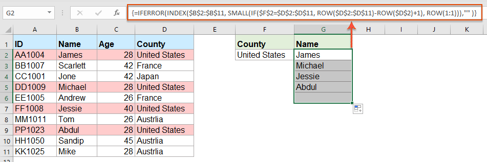
1. Copiați sau introduceți formula de mai jos într-o celulă goală unde doriți să localizați rezultatul:

=INDEX($B$2:$B$11, SMALL(IF(COUNTIF($F$2, $C$2:$C$11)*COUNTIF($G$2, $D$2:$D$11), ROW($A$2:$D$11)-MIN(ROW($A$2:$D$11))+1), ROW(A1)), COLUMN(A1))

notițe: În formula de mai sus, B2: B11 este coloana din care se returnează valoarea potrivită; F2, C2: C11 sunt prima condiție și datele coloanei care conține prima condiție; G2, D2: D11 sunt a doua condiție și datele coloanei care conțin această condiție, vă rugăm să le modificați în funcție de nevoile dvs.

2. Apoi, apăsați Ctrl + Shift + Enter tastele pentru a obține primul rezultat de potrivire, apoi selectați prima celulă de formulă și trageți mânerul de umplere în jos până la celule până când este afișată valoarea erorii, acum toate valorile de potrivire sunt returnate așa cum se arată în imaginea de mai jos:

sfaturi: Dacă trebuie doar să returnați toate valorile potrivite pe baza unei condiții, aplicați formula matricei de mai jos:

=IFERROR(INDEX($B$2:$B$11, SMALL(IF($F$2=$D$2:$D$11, ROW($D$2:$D$11)-ROW($D$2)+1), ROW(1:1))),"" )


Mai multe articole relative:

  • Returnează mai multe valori de căutare într-o singură celulă separată prin virgulă
  • În Excel, putem aplica funcția VLOOKUP pentru a returna prima valoare potrivită dintr-o celulă de tabel, dar, uneori, trebuie să extragem toate valorile potrivite și apoi să le separăm printr-un delimitator specific, cum ar fi virgulă, liniuță etc. într-o singură celulă după cum se arată în următoarea captură de ecran. Cum am putea obține și returna mai multe valori de căutare într-o singură celulă separată prin virgule în Excel?
  • Vizualizați și returnați mai multe valori de potrivire simultan în foaia Google
  • Funcția normală Vlookup din foaia Google vă poate ajuta să găsiți și să returnați prima valoare potrivită pe baza unor date date. Dar, uneori, poate fi necesar să căutați și să returnați toate valorile potrivite, după cum se arată în următoarea captură de ecran. Aveți vreo modalitate bună și ușoară de a rezolva această sarcină în foaia Google?
  • Vizualizați și returnați mai multe valori din lista derulantă
  • În Excel, cum ați putea să căutați și să returnați mai multe valori corespunzătoare dintr-o listă derulantă, ceea ce înseamnă că atunci când alegeți un articol din lista derulantă, toate valorile sale relative sunt afișate simultan, după cum se arată în următoarea captură de ecran. În acest articol, voi introduce soluția pas cu pas.
  • Vizualizați și returnați mai multe valori pe verticală în Excel
  • În mod normal, puteți utiliza funcția Vlookup pentru a obține prima valoare corespunzătoare, dar, uneori, doriți să returnați toate înregistrările de potrivire pe baza unui criteriu specific. În acest articol, voi vorbi despre cum să vizualizați și să returnați toate valorile potrivite pe verticală, orizontală sau într-o singură celulă.
  • Vlookup și returnează datele de potrivire între două valori în Excel
  • În Excel, putem aplica funcția normală Vlookup pentru a obține valoarea corespunzătoare pe baza datelor date. Dar, uneori, dorim să căutăm și să returnăm valoarea potrivită între două valori așa cum se arată în următoarea captură de ecran, cum ați putea face față acestei sarcini în Excel?


  • Super Formula Bar (editați cu ușurință mai multe linii de text și formulă); Layout de citire (citiți și editați cu ușurință un număr mare de celule); Lipiți la interval filtrat...
  • Merge celule / rânduri / coloane și păstrarea datelor; Conținut de celule divizate; Combinați rânduri duplicate și sumă / medie... Prevenirea celulelor duplicate; Comparați gamele...
  • Selectați Duplicat sau Unic Rânduri; Selectați Rânduri goale (toate celulele sunt goale); Super Find și Fuzzy Find în multe cărți de lucru; Selectare aleatorie ...
  • Copie exactă Mai multe celule fără modificarea referinței formulelor; Creați automat referințe la foi multiple; Introduceți gloanțe, Casete de selectare și multe altele ...
  • Formule favorite și inserare rapidă, Gama, Diagrame și Imagini; Criptați celulele cu parola; Creați o listă de corespondență și trimiteți e-mailuri ...
  • Extrageți textul, Adăugați text, eliminați după poziție, Eliminați spațiul; Creați și imprimați subtotaluri de paginare; Convertiți conținutul dintre celule și comentarii...
  • Super Filtru (salvați și aplicați scheme de filtrare altor foi); Sortare avansată după lună / săptămână / zi, frecvență și multe altele; Filtru special cu bold, italic ...
  • Combinați cărți de lucru și foi de lucru; Merge Tables pe baza coloanelor cheie; Împărțiți datele în mai multe foi; Conversia în loturi xls, xlsx și PDF...
  • Gruparea tabelului pivot după numărul săptămânii, ziua săptămânii și multe altele ... Afișați celulele deblocate, blocate prin diferite culori; Evidențiați celulele care au formulă / nume...
fila kte 201905
  • Activați editarea și citirea cu file în Word, Excel, PowerPoint, Publisher, Access, Visio și Project.
  • Deschideți și creați mai multe documente în filele noi ale aceleiași ferestre, mai degrabă decât în ​​ferestrele noi.
  • Vă crește productivitatea cu 50% și reduce sute de clicuri de mouse pentru dvs. în fiecare zi!
fundul officetab


Comments (25)
No ratings yet. Be the first to rate!
This comment was minimized by the moderator on the site
Hi, if there are duplicate values (e.g. two adams), how do i make sure that it only returns 1 adam and not 2?
This comment was minimized by the moderator on the site
Hello, Bobby,
To extract only unique matching values, you should apply the below formula:
After pasting the formula, please press Ctrl + Shift + Enter keys together to get the correct result.
=IFERROR(INDEX($B$2:$B$5, MATCH(0, COUNTIF(H1:$H$1, $B$2:$B$5)+IF($D$2:$D$5<>$G$2, 1, 0)+IF($C$2:$C$5<>$F$2, 1, 0), 0)), "")

Please have a try, hope it can help you!
This comment was minimized by the moderator on the site
Hi,

Thanks for posting these examples.
I'm trying to implement this in my own sheet, but don't get it to work (maybe because I'm using an europe version of excel)?

I want to get the dates of the days that I had my shifts or that I have worked 'some' (>0) hours for a client.

So in I3 is the name and in J3 the month. K3 and L3 are the shifts (1 is worked) and hours (don't know how to set this, should be more than zero)

My expected results are in:
Shifts: I7 and I8
hours: J7

So I worked more than 0 hours for 'person 2' in oktober on 3-10-2022
had shifts for person 2 on '10-10-2022' and 28-10-2022

When I add '=INDEX($B$2:$B$11, SMALL(IF(COUNTIF($F$2, $C$2:$C$11)*COUNTIF($G$2, $D$2:$D$11), ROW($A$2:$D$11)-MIN(ROW($A$2:$D$11))+1), ROW(A1)), COLUMN(A1))' in my excel sheet, it doesn't allow the comma between the different parts of the formula.
So I need to change them to ';'.
But when I try it it always says: '#NAME?'

So can someone help me with this?

Kind regards,

Bas
[img]https://drive.google.com/file/d/1iIPQKuj_PNhqWyWlwJ4IQTqGNEd6B9Hw/view?usp=share_link[/img]
This comment was minimized by the moderator on the site
Hi,

First, thank you for sharing!

Can you please provide a solution to the case below:

I have 3 columns (A: Containing reference information, B: Containing information to be searched, C: Search result)

Image url is provided below

https://ibb.co/VHCd09K

Column A-------------------------Column B------------Column C
File Name-------------------------Name----------------File Name, Document Name, Element Name, Name
Changed Element-----------------Element--------------Changed Element, Element Name, Element ID
Column Location
Document Name
Element Name
Name
Category
Warranty
Slope
Element ID

What I need is to search in column A for any partial match with cell B2 (Name) or B3 (Element) and get the result in one cell,

Thank you, Behzad
This comment was minimized by the moderator on the site
Hello, Behzad
Maybe the below User Defined Function can help you.
Public Function ConcatPartLookUp(rngInput As Range, rngSource As Range, Optional strDelimiter As String, Optional blCaseSensitive)
Dim rng As Range
If strDelimiter = "" Then strDelimiter = ","
If IsMissing(blCaseSensitive) Then
    blCaseSensitive = False
Else
    blCaseSensitive = True
End If
For Each rng In rngSource
    If blCaseSensitive Then
        If InStr(1, rng.Value, rngInput.Value, vbBinaryCompare) > 0 Then ConcatPartLookUp = ConcatPartLookUp & strDelimiter & rng.Value
    Else
        If InStr(1, rng.Value, rngInput.Value, vbTextCompare) > 0 Then ConcatPartLookUp = ConcatPartLookUp & strDelimiter & rng.Value
    End If
Next
If Len(ConcatPartLookUp) > 0 Then ConcatPartLookUp = Mid(ConcatPartLookUp, 2, Len(ConcatPartLookUp))
End Function


After copying and pasting this code, and then use this formula:=ConcatPartLookUp(B2,$A$2:$A$8) to get the result you need.
Please have a try, hope it can help you!
This comment was minimized by the moderator on the site
Heyi, thank you for the formula. It worked for "fixed" values / text as criterias. However, one of the criterias i'm trying to use is a condition (values <>0 ), but does not work the described formula. Do you guys know what should i change to adapt the formula so I can have a condition as one of the criterias, please?

Best,

João
This comment was minimized by the moderator on the site
Hello, Marcus
To solve your problem, please view this article:
https://www.extendoffice.com/documents/excel/6393-excel-vlookup-function.html#b3-2
There are some detailed explanations of this task. You just need to change the criteira to your own.
Thank you!
This comment was minimized by the moderator on the site
Hi,

if in cell H1 i write "Name" and wanted to link that with the formula, how would that work?
Then I could write "ID" in cell H1 and would automatically get as a result: AA1004; DD1009; PP1023 (for the first formula)

Thank you in advance!
This comment was minimized by the moderator on the site
Hello, Marie
Sorry, i can't get the point of your first problem, could you explain your problem more clearly and detailedly? Or you can insert a screenshot here to describe your problem.
As for the second question, you just need to change the cell reference as this:
=INDEX($A$2:$A$11, SMALL(IF(COUNTIF($F$2, $C$2:$C$11)*COUNTIF($G$2, $D$2:$D$11), ROW($A$2:$D$11)-MIN(ROW($A$2:$D$11))+1), ROW(A1)), COLUMN(A1))

Remeber to press Ctrl + Shift + Enter keys together.
Please try, hope it can help you!
This comment was minimized by the moderator on the site
Hello,
what would be needed to expand the first formula in the following case:
Some IDs are Blank (e.g. cell A5 is blank) and I would like an additional condition outputting lines only when the IDs are not blank. (So the output should then be James and Abdul.
Thanks!
This comment was minimized by the moderator on the site
Hello, Jo,
To solve your problem, please apply the below formula:
=INDEX($B$2:$B$11, SMALL(IF(COUNTIF($F$2, $C$2:$C$11)*COUNTIF($G$2, $D$2:$D$11)*($A$2:$A$11<>0), ROW($A$2:$D$11)-MIN(ROW($A$2:$D$11))+1), ROW(A1)), COLUMN(A1))

Please have a ry, hope it can help you!
This comment was minimized by the moderator on the site
hello,
ive tried using the formula and it either generates a value of 0 or the image attached
This comment was minimized by the moderator on the site
Hello, Milku
Your screenshot showed WPS software of MAC version, so I am not sure whether our formula is available.
I uploaded an Excel file to here, you can try to see if it can calculate correctly in you environment.
Thank you!
This comment was minimized by the moderator on the site
When I use the second formula and drag down, nothing appears. The formula result (fx) says it should be returning something but it is blank. How do I correct this?
This comment was minimized by the moderator on the site
Hello Alysia,

Glad to help. I tried the second formula in the article and drag the formula down, the rest of results were returned. I think there may be two reasons for your problem. First, maybe you forget to press Ctrl + Shift + Enter keys to enter the formula. Second, the matching result is only one, so no other results are not returned. Please have a check.

Sincerely,
Mandy
This comment was minimized by the moderator on the site
Hi,

I was wondering if it at all possible to enter a 2nd criteria but from the same range as the 1st criteria,

For example with the used example above i would like to search for the names of people from both America and France So cell F3 would have France, Scarlett & Andrew would also populate in the list in Column G

Thank you for assistance in advance.
This comment was minimized by the moderator on the site
Hello Nick,

Glad to help. If you want to get the names of people from both America and France, I advise you to use our formula twice to get the result. Please see the screenshot, In F2 and G2 are values "United States" and "France". Apply formula =IFERROR(INDEX($B$2:$B$11, SMALL(IF($F$2=$D$2:$D$11, ROW($D$2:$D$11)-ROW($D$2)+1), ROW(1:1))),"" ) to get the results for America. And apply formula =IFERROR(INDEX($B$2:$B$11, SMALL(IF($G$2=$D$2:$D$11, ROW($D$2:$D$11)-ROW($D$2)+1), ROW(1:1))),"" ) to get the results for France. It's simple. Please have a try.

Sincerely,
Mandy
This comment was minimized by the moderator on the site
In the first example, what change to the formula would be needed to return everyone who was less than 28 years old?
There are no comments posted here yet
Load More
Please leave your comments in English
Posting as Guest
×
Rate this post:
0   Characters
Suggested Locations